Software Quality Metrics

Here, the goals of software measurement are to answer, among others, the following questions:

• Is it possible to predict the error-proneness of a system using software measures from its design phase.

• Is it possible to extract quantitative features from the representation of a software design to enable us to predict the degree of maintainability of a software system.

• Are there any quantifiable, key features of the program code of a module that would enable us to predict the degree of difficulty of testing for that module, and the number of residual errors in the module after a particular level of testing has occurred.

• Is it possible to extract quantifiable features from the representation of a software design to enable us to predict the amount of effort required to build the software described by that design.

• Are there quantifiable features that can be extracted from the program code of a subroutine that can be used to help predict the amount of effort required to test the subroutine.

• Are there features in order to predict the size of a project from the specification phase.

• What properties of software measures are required in order to determine the quality of a design.

• What are the right software measures to underlie the software quality attributes of the ISO 9126 norm by numbers

The major question for people who want to use software measures or using software measures is: what are the benefits of software measurement for practitioners. Software measures re used to measure specific attributes of a software product or software development process

We use software measures to derive:

• A basis for estimates,

• To track project progress,

• To determine (relative) complexity,

• To help us to understand when we have archived a desired state of quality,

• To analyze or defects,

• and to experimentally validate best practices.

In short: they help us to make better decisions.

2. Definitions

For the purposes of this standard, the following terms and definitions apply. IEEE Std 100-1996 and IEEE Std 610.12-1990 should be referenced for terms not defined in this clause.

2.1 attribute: A measurable physical or abstract property of an entity.

2.2 critical range: Metric values used to classify software into the categories of acceptable, marginal, or unacceptable.

2.3 critical value: Metric value of a validated metric that is used to identify software that has unacceptable quality.

2.4 direct metric: A metric that does not depend upon a measure of any other attribute.

2.5 direct metric value: A numerical target for a quality factor to be met in the final product. For example, mean time to failure (MTTF) is a direct metric of final system reliability.

2.6 measure: (A) A way to ascertain or appraise value by comparing it to a norm. (B) To apply a metric.

2.7 measurement: The act or process of assigning a number or category to an entity to describe an attribute of that entity. A figure, extent, or amount obtained by measuring.

2.8 metric: See: software quality metric.

NOTE The term metric is used in place of the term software quality metric.

2.9 metrics framework: A decision aid used for organizing, selecting, communicating, and evaluating the required quality attributes for a software system. A hierarchical breakdown of quality factors, quality sub-factors, and metrics for a software system.

2.10 metrics sample: A set of metric values that is drawn from the metrics database and used in metrics validation.

2.11 metric validation: The act or process of ensuring that a metric reliably predicts or assesses a quality factor.

2.12 metric value: A metric output or an element that is from the range of a metric.

2.13 predictive metric: A metric applied during development and used to predict the values of a software quality factor.

2.14 predictive metric value: A numerical target related to a quality factor to be met during system development. This is an intermediate requirement that is an early indicator of final system performance. For example, design or code errors may be early predictors of final system reliability.

2.15 process metric: A metric used to measure characteristics of the methods, techniques, and tools employed in developing, implementing, and maintaining the software system

2.16 product metric: A metric used to measure the characteristics of any intermediate or Þnal product of the software development process.

2.17 quality attribute: A characteristic of software, or a generic term applying to quality factors, quality subfactors, or metric values.

2.18 quality factor: A management-oriented attribute of software that contributes to its quality.

2.19 quality factor sample: A set of quality factor values that is drawn from the metrics database and used in metrics validation.

2.20 quality factor value: A value of the direct metric that represents a quality factor. See also: metric value.

2.21 quality requirement: A requirement that a software attribute be present in software to satisfy a contract, standard, specification, or other formally imposed document.

2.22 quality subfactor: A decomposition of a quality factor or quality subfactor to its technical components.

2.23 software component: A general term used to refer to a software system or an element, such as module, unit, data, or document.

2.24 software quality metric: A function whose inputs are software data and whose output is a single numerical value that can be interpreted as the degree to which software possesses a given attribute that affects its quality.

2.25 validated metric: A metric whose values have been statistically associated with corresponding quality factor values.

3. Software quality metrics framework (informative)

Software quality is the degree to which software possesses a desired combination of quality attributes. The purpose of software metrics is to make assessments throughout the software life cycle as to whether the software quality requirements are being met. The use of software metrics reduces subjectivity in the assessment and control of software quality by providing a quantitative basis for making decisions about software quality.

However, the use of software metrics does not eliminate the need for human judgment in software assessments. The use of software metrics within an organization or project is expected to have a beneficial effect by making software quality more visible.

More specifically, the use of this standards methodology for measuring quality enables an organization to:

• Assess achievement of quality goals;

• Establish quality requirements for a system at its outset;

• Establish acceptance criteria and standards;

• Evaluate the level of quality achieved against the established requirements;

• Detect anomalies or point to potential problems in the system;

• Predict the level of quality that will be achieved in the future;

• Monitor changes in quality when software is modified;

• Assess the ease of change to the system during product evolution;

• Validate a metrics set.

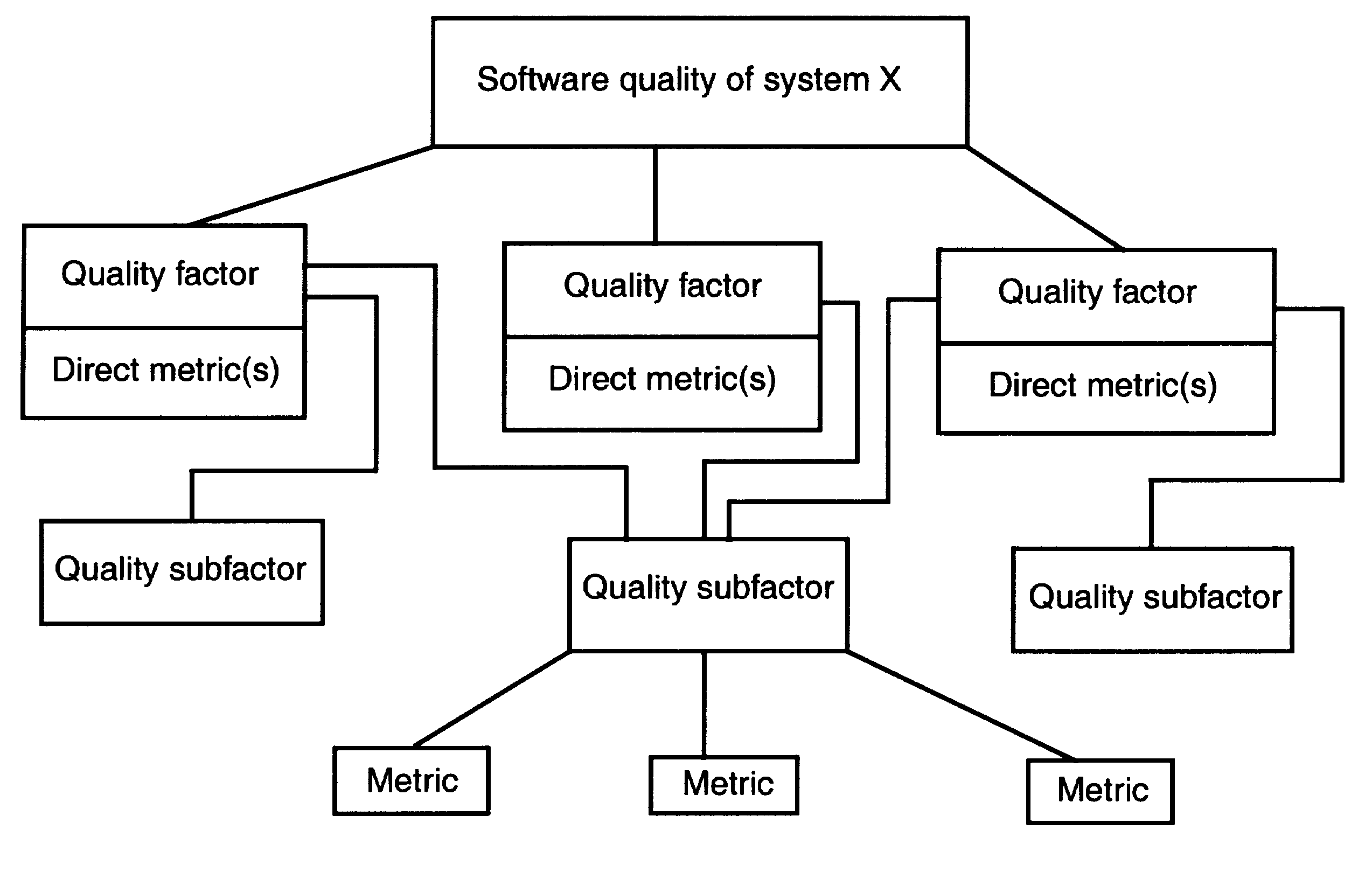
The software quality metrics framework shown in Figure 1 is designed to be flexible. It permits additions, deletions, and modifications of quality factors, quality subfactors, and metrics. Each level may be expanded to several sub levels. The framework can thus be applied to all systems and can be adapted as appropriate without changing the basic concept.

Figure 1 Software quality metrics framework

The first level of the software quality metrics framework hierarchy begins with the establishment of quality requirements by the assignment of various quality attributes, which are used to describe the quality of the entity system X. All attributes defining the quality requirements are agreed upon by the project team, and then the definitions are established. Quality factors that represent management and user-oriented views are then assigned to the attributes. If necessary, quality sub factors are then assigned to each quality factor. Associated with each quality factor is a direct metric that serves as a quantitative representation of a quality factor. For example, a direct metric for the factor reliability could be mean time to failure (MTTF). Identify one or more direct metrics and target values to associate with each factor, such as an execution time of 1 hour, that is set by project management. Otherwise, there is no way to determine whether the factor has been achieved.

At the second level of the hierarchy are the quality subfactors that represent software-oriented attributes that indicate quality. These can be obtained by decomposing each quality factor into measurable software attributes. Quality subfactors are independent attributes of software, and therefore may correspond to more than one quality factor. The quality subfactors are concrete attributes of software that are more meaningful than quality factors to technical personnel, such as analysts, designers, programmers, testers, and maintainers. The decomposition of quality factors into quality subfactors facilitates objective communication between the manager and the technical personnel regarding the quality objectives.

At the third level of the hierarchy the quality subfactors are decomposed into metrics used to measure system products and processes during the development life cycle. Direct metric values, or quality factor values, are typically unavailable or expensive to collect early in the software life cycle.

From top to bottom the framework facilitates:

• Establishment of quality requirements, in terms of quality factors, by managers early in a system's life cycle;

• Communication of the established quality factors, in terms of quality subfactors, to the technical personnel;

• Identification of metrics that are related to the established quality factors and quality subfactors.

From bottom to top the framework enables the managerial and technical personnel to obtain feedback by

• Evaluating the software products and processes at the metrics level;

• Analyzing the metric values to estimate and assess the quality factors.

4. The software quality metrics methodology

The software quality metrics methodology is a systematic approach to establishing quality requirements and identifying, implementing, analyzing, and validating the process and product software quality metrics for a software system. It comprises five steps (see 4.1 through 4.5).

These steps are intended to be applied iteratively because insights gained from applying a step may show the need for further evaluation of the results of prior steps. Each step states the activities needed to accomplish the indicated results.

4.1 Establish software quality requirements

The result of this step is a list of the quality requirements. The activities to accomplish this result are given in 4.1.1 through 4.1.3.

4.1.1 Identify a list of possible quality requirements

Identify quality requirements that are applicable to the software system. Use organizational experience, required standards, regulations, or laws to create this list. In addition, list other system requirements that may affect the feasibility of the quality requirements. Consider contractual requirements and acquisition concerns, such as cost or schedule constraints, warranties, customer metrics requirements, and organizational self-interest. Do not rule out mutually exclusive requirements at this point. Focus on quality factor/direct metric combinations instead of predictive metrics.

Ensure that all parties involved in the creation and use of the system participate in the quality requirements identification process.

4.1.2 Determine the list of quality requirements

Rate each of the listed quality requirements by importance. Determine the list of the possible quality requirements by doing the following:

a) Survey all involved parties. Discuss the relative priorities of the requirements with all involved parties. Have each group weigh the quality requirements against the other system requirements and constraints. Ensure that all viewpoints are considered.

b) Create the list of quality requirements. Resolve the results of the survey into a single list of quality requirements. The proposed quality factors for this list may have cooperative or conflicting relationships. Resolve any conflicts among requirements at this point. In addition, if the choice of quality requirements is in conflict with cost, schedule, or system functionality, alter one or the other.

Exercise care in choosing the desired list to ensure that the requirements are technically feasible, reasonable, complementary, achievable, and verifiable. Obtain agreement by all parties to this final list.

4.1.3 Quantify each quality factor

For each quality factor, assign one or more direct metrics to represent the quality factor, and assign direct metric values to serve as quantitative requirements for that quality factor. For example, if high efficiency was one of the quality requirements from 4.1.2, assign a direct metric (e.g., actual resource utilization/ allocated resource utilization with a value of 90%). Use direct metrics to verify the achievement of the quality requirements.

The quantified list of quality requirements and their definitions again is approved by all involved parties.

4.2 Identify software quality metrics

The result of this step is an approved metrics set. The activities to accomplish this result are given in 4.2.1 through 4.2.3.

4.2.1 Apply the software quality metrics framework

The quantified list of quality requirements and their definitions again is approved by all involved parties. Create a chart of the quality requirements based on the hierarchical tree structure found in Figure 1. At this

point, complete only the quality factor level. Next, decompose each quality factor into quality subfactors as indicated in Clause 3. Continue the decomposition into quality subfactors for as many levels as needed until the quality subfactor level is complete.

Using the software quality metrics framework, decompose the quality subfactors into metrics. For each validated metric on the metric level, assign a target value and a critical value and range that should be achieved during development.

Have the framework revised and the target values for the metrics reviewed and approved by all involved parties.

Use only validated metrics (i.e., either direct metrics or metrics validated with respect to direct metrics) to assess current and future product and process quality (see 4.5 for a description of the validation methodology). Retain non-validated metrics as candidates for future analysis. Furthermore, use only metrics that are associated with the quality requirements of the software project.

Document each metric using the format shown in Table 1.

4.2.2 Perform a cost-benefit analysis

4.2.2.1 Identify the costs of implementing the metrics

Identify and document (see Table 1) all the costs associated with each metric in the metrics set. For each metric, estimate and document the following costs and impacts:

a) Metrics utilization costs incurred by collecting data; automating metrics calculations; and applying, interpreting, and reporting the results;

b) Software change costs incurred by changing the development process;

c) Organizational structure change costs incurred by producing the software;

d) Special equipment required to implement the metrics plan;

e) Training required to implement the metrics plan.

Table 1 Metrics set

4.2.2.2 Identify the benefits of applying the metrics

Identify and document the benefits that are associated with each metric in the metrics set (see Table 1). Benefits to consider include the following:

a) Identify quality goals and increase awareness of the goals.

b) Provide timely feedback of quality problems to the development process.

c) Increase customer satisfaction by quantifying the quality of the software before it is delivered.

d) Provide a quantitative basis for making decisions about software quality.

e) Reduce software life cycle costs by improving process efficiency.

4.2.2.3 Adjust the metrics set

Weigh the benefits, tangible and intangible, against the costs of each metric. If the costs exceed the benefits of a given metric, alter or delete it from the metrics set. On the other hand, for metrics that remain, make plans for any necessary changes to the software development process, organizational structure, tools, and training. In most cases it will not be feasible to quantify benefits. In these cases, exercise judgment in weighing qualitative benefits against quantitative costs.

4.2.3 Gain commitment to the metrics set

Have all involved parties review the adjusted metrics. Have the metrics set adopted and supported by this group.

4.3 Implement the software quality metrics

The outputs of this step are a description of the data items, a traceability matrix, and a training plan and schedule. The activities to accomplish this result are given in 4.3.1 through 4.3.3.

4.3.1 Define the data collection procedures

For each metric in the metrics set, determine the data that will be collected and determine the assumptions that will be made about the data (e.g., random sample and subjective or objective measure).

Show the flow of data from point of collection to evaluation of metrics.

Identify tools and describe how they will be used.

Describe data storage procedures.

Establish a traceability matrix between metrics and data items.

Identify the organizational entities that will participate in data collection, including those responsible for monitoring data collection.

Describe the training and experience required for data collection and the training process for personnel involved.

Describe each data item thoroughly, using the format shown in Table 2.

4.3.2 Prototype the measurement process

Test the data collection and metrics computation procedures on selected software that will act as a prototype. Select samples that are similar to the project(s) on which the metrics will be used. Make an analysis to deter mine if the data are collected uniformly and if instructions have been interpreted consistently. In particular, check data that require subjective judgments to determine if the descriptions and instructions are clear enough to ensure uniform results.

Examine the cost of the measurement process for the prototype to verify or improve the cost analysis.

Use the results collected from the prototype to improve the metric descriptions (see Table 1) and descriptions of data items (see Table 2).

4.3.3 Collect the data and compute the metric values

Using the formats in Tables 1 and 2, collect and store data in the project metrics database at the appropriate time in the life cycle. Check the data for accuracy and proper unit of measure.

Table 2 Data item description

Monitor the data collection. If a sample of data is used, verify that requirements such as randomness, minimum size of sample, and homogeneous sampling have been met. Check for uniformity of data if more than one person is collecting it.

Compute the metric values from the collected data.

4.4 Analyze the software metrics results

The results of this step are changes to the organization and development process, which are indicated from interpreting and using the measurement data. The activities to accomplish this result are given in 4.4.1 through 4.4.4.

4.4.1 Interpret the results

Interpret and record the results. Analyze the differences between the collected metric data and the target values. Investigate significant differences.

4.4.2 Identify software quality

Identify and review quality metric values for software components. Identify quality metric values that are outside the anticipated tolerance intervals (low or unexpected high quality) for further study. Unacceptable quality may be manifested as excessive complexity, inadequate documentation, lack of traceability, or other undesirable attributes. The existence of such conditions is an indication that the software may not satisfy quality requirements when it becomes operational. Because many of the direct metrics that are usually of interest cannot be collected during software development (e.g., reliability metrics), use validated metrics when direct metrics are not available. Use direct or validated metrics for software components and process steps. Compare metric values with critical values of the metrics. Analyze in detail software components whose values deviate from the critical values. Depending on the results of the analysis, redesign (acceptable quality is achieved by redesign), scrap (quality is so poor that redesign is not feasible), or do not change (deviations for critical metric values are judged to be insignificant) the software components.

4.4.3 Make software quality predictions

Use validated metrics during development to make predictions of direct metric values. Compare predicted values of direct metrics with target values to determine whether to flag software components for detailed analysis. Make predictions for software components and process steps. Analyze in detail software components and process steps whose predicted direct metric values deviate from the target values.

4.4.4 Ensure compliance with requirements

Use direct metrics to ensure compliance of software products with quality requirements during system and acceptance testing. Use direct metrics for software components and process steps. Compare these metric values with target values of the direct metrics. Classify software components and process steps whose measurements deviate from the target values as non-compliant.

4.5 Validate the software quality metrics

The result of this step is a set of validated metrics for making predictions of quality factor values. The activities to accomplish this result are given in 4.5.1 through 4.5.3.

4.5.1 Apply the validation methodology

The purpose of metrics validation is to identify both product and process metrics that can predict specified quality factor values, which are quantitative representations of quality requirements. Metrics shall indicate whether quality requirements have been achieved or are likely to be achieved in the future. When it is possible to measure quality factor values at the desired point in the life cycle, direct metrics shall be used to evaluate software quality. At some points in the life cycle, certain quality factor values (e.g., reliability) are not available. They are obtained after delivery or late in the project. In these cases, validated metrics shall be used early in a project to predict quality factor values.

Validation does not mean a universal validation of the metrics for all applications. Rather it refers to validating the relationship between a set of metrics and a quality factor for a given application.

The history of the application of metrics indicates that predictive metrics were seldom validated (i.e., it was not demonstrated through statistical analysis that the metrics measured software characteristics that they purported to measure). However, it is important that predictive metrics be validated before they are used to evaluate software quality. Otherwise, metrics might be misapplied (i.e., metrics might be used that have little or no relationship to the desired quality characteristics).

Although quality subfactors are useful when identifying and establishing quality factors and metrics, they are not used in metrics validation, because the focus in validation is on determining whether a statistically significant relationship exists between predictive metric values and quality factor values.

Quality factors may be affected by multiple variables. A single metric, therefore, may not sufficiently represent any one quality factor if it ignores these other variables.

4.5.2 Apply validity criteria

To be considered valid, a predictive metric shall have a high degree of association with the quality factors it represents by conforming to the thresholds listed below. A metric may be valid with respect to certain validity criteria and invalid with respect to other criteria. For the purpose of assessing whether a metric is valid, the following thresholds shall be designated:

V - square of the linear correlation coefficient

B - rank correlation coefficient

A - prediction error

𝜶 - confidence level

P - success rate

The description of each validity criterion is given below. For a numerical example of metrics validation calculations, see Annex B.

a) Correlation. The variation in the quality factor values explained by the variation in the metric values, which is given by the square of the linear correlation coefficient (R²) between the metric and the corresponding quality factor, shall exceed V.

This criterion assesses whether there is a sufficiently strong linear association between a quality factor and a metric to warrant using the metric as a substitute for the quality factor, when it is infeasible to use the latter.

b) Tracking. If a metric M is directly related to a quality factor F, for a given product or process, then a change in a quality factor value from F _T1 to F _T2 , at times T₁ and T_2, shall be accompanied by a change in metric value from M _T1 to M _T2 . This change shall be in the same direction (e.g., if F increases, M increases). If M is inversely related to F, then a change in F shall be accompanied by a change in M in the opposite direction (e.g., if F increases, M decreases). To perform this test, compute the coefficient of rank correlation (r) from n paired values of the quality factor and the metric.

Each of the quality factor/metric pairs shall be measured at the same point in time, and the n pairs of values are measured at n points in time. The absolute value of r shall exceed B. This criterion assesses whether a metric is capable of tracking changes in product or process quality over the life cycle.

c) Consistency. If quality factor values F₁ , F₂ , F_n , corresponding to products or processes 1, 2, n, have the relationship F₁ > F₂ > F_n , then the corresponding metric values shall have the relationship M ₁ > M ₂ > M _n . To perform this test, compute the coefficient of rank correlation (r) between paired values (from the same software components) of the quality factor and the metric. The absolute value of r shall exceed B.

This criterion assesses whether there is consistency between the ranks of the quality factor values of a set of software components and the ranks of the metric values for the same set of software components. This criterion shall be used to determine whether a metric can accurately rank, by quality, a set of products or processes.

d) Predictability. If a metric is used at time T₁ to predict a quality factor for a given product or process, it shall predict a related quality factor Fp_T2 with an accuracy of

(1)

where

Fa_T2 is the actual value of F at time T2.

This criterion assesses whether a metric is capable of predicting a quality factor value with the required accuracy.

e) Discriminative power. A metric shall be able to discriminate between high-quality software components (e.g., high MTTF) and low-quality software components (e.g., low MTTF). The set of metric values associated with the former should be significantly higher (or lower) than those associated with the latter.

This criterion assesses whether a metric is capable of separating a set of high-quality software components from a set of low-quality components. This capability identified critical values for metrics that shall be used to identify software components that have unacceptable quality. To perform this test, put the quality factor and metric data in the form of a contingency table and compute the chi-square statistic. This value shall exceed the chi-square statistic corresponding to 𝝰.

f) Reliability. A metric shall demonstrate the correlation, tracking, consistency, predictability, and discriminative power properties for at least P% of the applications of the metric.

This criterion is used to ensure that a metric has passed a validity test over a sufficient number or percentage of applications so that there shall be confidence that the metric can perform its intended function consistently.

4.5.3 Validation procedure

4.5.3.1 Identify the quality factors sample

A sample of quality factors shall be drawn from the metrics database.

4.5.3.2 Identify the metrics sample

A sample from the same domain (e.g., same software components), as used in 4.5.3.1, shall be drawn from the metrics database.

4.5.3.3 Perform a statistical analysis

The analysis described in 4.5.2 shall be performed.

Before a metric is used to evaluate the quality of a product or process, it shall be validated against the criteria described in 4.5.2. If a metric does not pass all of the validity tests, it shall only be used according to the criteria prescribed by those tests (e.g., if it only passes the tracking validity test, it shall be used only for tracking the quality of a product or process).

4.5.3.4 Document the results

Documented results shall include the direct metric, predictive metric, validation criteria, and numerical results, as a minimum.

4.5.3.5 Re-validate the metrics

A validated metric may not necessarily be valid in other environments or future applications. Therefore, a predictive metric shall be revalidated before it is used for another environment or application.

4.5.3.6 Evaluate the stability of the environment

Metrics validation shall be undertaken in a stable development environment (i.e., where the design language, implementation language, or project development tools do not change over the life of the project in which validation is performed). An organization initiates conformance to the validation requirements of this standard by collecting and validating metrics on a project (the validation project). This project shall be similar to the one in which the metrics are applied (the application project) with respect to software engineering skills, application, size, and software engineering environment.

Validation and application of metrics shall be performed during the same life cycle phases on different projects. For example, if metric X is collected during the design phase of project A and later validated with respect to quality factor Y, which is collected during the operations phase of project A, metric X would be used during the design phase of project B to predict quality factor Y with respect to the operations phase of project B.

Annex A

(informative)

Additional frameworks

This annex describes additional frameworks that could be considered in establishing a metrics framework in an organization.

A.1 Goal/question/metric (GQM) paradigm

The GQM paradigm is a mechanism for defining and evaluating a set of operational goals, using measurement. It represents a systematic approach to tailoring and integrating goals with models of the software processes, products, and quality perspectives of interest, based upon the specific needs of the project and the organization.

The goals are defined in an operational, tractable way by refining them into a set of quantifiable questions that are used to extract the appropriate information from the models. The questions and models, in turn, define a specific set of metrics and data for collection and provide a framework for interpretation.

The GQM paradigm was originally developed for evaluating defects for a set of projects in the National Aeronautics and Space Administration (NASA)/Goddard Space Flight Center (GSFC) environment. The application involved a set of case study experiments. It was then expanded to include various types of experimental approaches, including controlled experiments.

Although the GQM paradigm was originally used to define and evaluate goals for a particular project in a particular environment, its use has been expanded to a larger context. It is used as the goal-setting step in an evolutionary improvement paradigm tailored for a software development organization, the Quality Improvement Paradigm (QIP), and an organizational approach for building software competencies and supplying them to projects, the Experience Factory (EF).

Applying the GQM paradigm involves

a) Developing a set of corporate, division, and project goals for productivity and quality (e.g., customer satisfaction, on-time delivery, and improved quality);

b) Generating questions (based upon models) that define those goals as completely as possible in a quantifiable way;

c) Specifying the measures needed to be collected to answer those questions and to track process and product conformance to the goals;

d) Developing mechanisms for data collection;

e) Collecting, validating, and analyzing the data in real time to provide feedback to projects for corrective action, and analyzing the data in a post-mortem fashion to assess conformance to the goals and make recommendations for future improvements.

The process of setting goals and refining them into quantifiable questions is complex and requires experience. In order to support this process, a set of templates for setting goals, and a set of guidelines for deriving questions and metrics have been developed. These templates and guidelines reflect the GSFC experience from having applied the GQM paradigm in a variety of environments. The current set of templates and guidelines represent our current thinking and well may change over time as experience grows.

Goals may be defined for any object, for a variety of reasons, with respect to various models of quality, from various points of view, relative to a particular environment. The goal is defined by filling in a set of values for the various parameters in the template. Template parameters include purpose (what object and why), perspective (what aspect and who), and the environmental characteristics (where).

• Purpose: Analyze some (objects: processes, products, other experience models) for the purpose of (why: characterization, evaluation, prediction, motivation, improvement)

• Perspective: with respect to (what aspect: cost, correctness, defect removal, changes, reliability, user friendliness, etc.) from the point of view of (who: user, customer, manager, developer, corporation,etc.)

• Environment: in the following context: (where: problem factors, people factors, resource factors, process factors, etc.)

Example: Analyze the (system testing method) for the purpose of (evaluation) with respect to a model of (defect removal effectiveness) from the point of view of the (developer) in the following context: the standard NASA/GSFC environment, i.e., process model [e.g., Software Engineering Laboratory (SEL) version of the waterfall model], application (ground support software for satellites), machine, etc.

The purpose is meant to define the object or objects of study, what is going to be done, and why it is being done. There may be several objects and several purposes. It is clear that the author must avoid complex objectives. In some cases it may be wise to break a complex goal into several simpler goals.

The perspective is meant to define a particular angle or set of angles for evaluation. The author may choose more than one model, e.g., defects and changes, and more than one point of view, e.g., the corporation and the project manager. The author should define the model and assume the mind-set of the person who wants to know the information so that all aspects of the evaluation are performed from that point of view.

The purpose of the environment is to define the context of the study by defining all aspects of the project so it can be categorized correctly and the appropriate set of similar projects can be found as a basis of comparison. Types of quality factors include process factors, people factors, problem factors, methods, tools, and constraints. In general, the environment should include all those quality factors that may be common among all projects and become part of the database for future comparisons. Thus the environmental quality factors, rather than the values associated with these quality factors, should be consistent across several goals within the project and the organization. Some quality factors may have already been specified as part of the particular object or model under study and thus appear there in greater depth and granularity.

A.2 Practical software measurement (PSM)

This clause contains an overview of PSM. Software measurement does not replace other management skills and techniques. Neither does it operate in a vacuum. In particular, measurement enables the other quantitative disciplines of risk management and financial performance management. These three disciplines each have a planning and a tracking part.

While these disciplines are often promoted and implemented independently, the greatest value is derive from an integrated approach. Risk analysis helps to identify and prioritize issues that drive the definition of the measurement process. The measurement process helps quantify the likelihood and impact of risks. The measurement process provides an objective basis for reporting financial performance using techniques like earned value. Risks, status measures, and financial performance all need to be considered when making project decisions. Together, these three quantitative management disciplines complement traditional management skills and techniques.

How does an organization that wants to take advantage of the benefits of software measurement proceed? A number of specific measurement prescriptions have been offered to government and industry organizations with limited success. Rather than propose another fixed measurement scheme, PSM presents a flexible measurement approach. PSM views measurement as a process that must be adapted to the technical and management characteristics of each project. This measurement process is risk and issue driven. That is, it provides information about the specific risks, issues, and objectives important to project success.

The PSM approach defines three basic measurement activities necessary to get measurement into practice.

The first two activities, tailoring measures to address project information needs and applying measures to obtain insight into project risks and issues, are the basic subprocesses of the measurement process. The third activity, implementing measurement, includes the tasks necessary to establish this measurement process within an organization.

• The tailoring activity addresses the selection of an effective and economical set of measures for the project.

• The application activity involves collecting, analyzing, and acting upon the data defined in the tailoring activity. PSM recommends that these two activities be performed by a measurement analyst who is independent of the software developer.

• The implementation activity addresses the cultural and organizational changes necessary to establish a measurement process. Implementing a measurement process requires the support of project and organizational managers.

The measurement process must be integrated into the developer’s software process. The nature of the developer’s process determines the opportunities for measurement. Because the software process itself is dynamic, the measurement process also must change and adapt as the project evolves. This makes the activities of measurement tailoring and application iterative throughout the project life cycle. The issues, measures, and analysis techniques change over time to best meet the project’s information needs.

A.2.1 Principles

Each project is described by different management and technical characteristics, and by a specific set of software risks and issues. To address the unique measurement requirements of each project, PSM explains how to tailor and apply a generally defined software measurement process to meet specific project information needs. To help do this, PSM provides nine principles that define the characteristics of an effective measurement process. These principles are based upon actual measurement experience on successful projects.

a) Project risks, issues, and objectives drive the measurement requirements.

b) The developer’s process defines how the software is actually measured.

c) Collect and analyze data at a level of detail sufficient to identify and isolate problems.

d) Implement an independent analysis capability.

e) Use a structured analysis process to trace the measures to the decisions.

f) Interpret the measurement results in the context of other project information.

g) Integrate software measurement into the project management process throughout the software life cycle.

h) Use the measurement process as a basis for objective communication.

I) Focus initially on single project analysis.

Experience has shown that a measurement process that adheres to these principles is more likely to succeed.

A.2.2 Issues

The purpose of software measurement is to help management achieve project objectives, identify and track risks, satisfy constraints, and recognize problems early. These management concerns are referred to, collectively, as issues. Note that issues are not necessarily problems, but rather they define areas where problems may occur. An initial set of issues are identified at the outset of the project. This issue set evolves and changes as the project progresses. Almost all issues can be expressed as risks. Conducting a thorough risk analysis at project outset facilitates measurement implementation. However, even if a formal risk analysis has not been performed, issues still can be identified.

PSM emphasizes identifying project issues at the start of a project and then using the measurement process to provide insight to those issues. While some issues are common to most or all projects, each project typically has some unique issues. Moreover, the priority of issues usually varies from project to project.

The six common software issues addressed in this standard are as follows:

a) Schedule and progress;

b) Resources and cost;

c) Growth and stability;

d) Product quality;

e) Development performance;

f) Technical adequacy.

These common issues may also be thought of as classes or categories of risks.

At the start of a project, or when major changes are implemented, each of these issues is analyzed in terms of the feasibility of the plan. For example, the project manager may ask questions such as, “Is this a reasonable size estimate?” or, “Can the software be completed with the proposed amount of effort and schedule?” Once the project is underway, the manager’s concern turns to performance. The key questions then become ones such as, “Is the project on schedule?” or, “Is the quality good enough?”

It is important to note that software issues are not independent. For example, requirements growth may result in schedule delays or effort overruns. Moreover, the impact of the addition of work to a project (size growth) may be masked, in terms of level of effort, by stretching out the schedule. Thus, it is important that issues be considered together, rather than individually, to get a true understanding of project status.

Focusing measurement attention on items that provide information about the project's issues also minimizes the effort required for the measurement process. Resources are not expended collecting data that may not get used.

Experience from a wide variety of commercial and government organizations shows that the cost of implementing and operating a measurement process as described in PSM ranges from 1% to 5% of the project's software budget. This is a relatively small amount when compared to the cost of conventional review- and documentation-based project-monitoring techniques.

Annex B

(informative)

Sample metrics validation calculations

B.1 Correlation validity criterion

Assume V, the square of the linear correlation coefficient, has been designated as 0.7 and the correlation coefficient between a complexity metric and the quality factor reliability is 0.9. The square of this is 0.81. Eighty one percent of the variation in the quality factor is explained by the variation in the metric. If this relationship is demonstrated over a representative sample of software components, conclude that the metric correlates with reliability.

B.2 Tracking validity criterion

Assume B, the rank correlation coefficient, has been designated as 0.7. Further assume that a complexity metric is a measure of reliability. Then a change in the reliability of a software component is accompanied by an appropriate change in the complexity metric’s value. For example, if the product increases in reliability, the metric value also changes in a direction that indicates the product has improved. Assume mean time to failure (MTTF) is used to measure reliability and is equal to 1000 hours during testing (T1) and 1500 hours during operation (T2). Also assume a complexity metric whose value is 8 in T1 and 6 in T2,where 6 is less complex than 8. Then complexity tracks reliability for this software component. Compute the coefficient of rank correlation r from n paired values of the quality factor and the metric over a representative sample of software components. If r exceeds 0.7, conclude that the metric tracks reliability (i.e., indicates changes in product reliability) over the software life cycle.

B.3 Consistency validity criterion

Assume B, the rank correlation coefficient, has been designated as 0.7. Further assume the reliability of software components X, Y, and Z, as measured by MTTF, is 1000 hours, 1500 hours, and 800 hours, respectively, and the corresponding complexity metric values are 5, 3, and 7, where low metric values are better than high values. Then the ranks for reliability and metric values, with 1 representing the highest rank, are as shown in Table B.1. Compute the coefficient of rank correlation r from n paired values of the quality factor and the metric over a representative sample of software components. If r exceeds 0.7, conclude that the metric is consistent and ranks the quality of software components. For example, the ranks establish priority of testing and allocation of budget and effort to testing (i.e., the worst software component receives the most attention, largest budget, and most staff).

Table B.1 Ranks for reliability and metric values

B.4 Predictability validity criterion

Assume A, the prediction error, has been designated as 25%. Further assume that a complexity metric is used during development at time T1 to predict the reliability of a software component during operation to be an MTTF of 1200 hours ( Fp_T2 ) at time T2. Also assume that the actual MTTF during operation is 1000 hours ( Fa_T2 ). Then the error in prediction is 200 hours, or 20%. Conclude that the prediction accuracy is acceptable. If the ability to predict is demonstrated over a representative sample of software components, conclude that the metric can be used as a predictor of reliability. For example, during development predictions identify those software components that need to be improved.

B.5 Discriminative power validity criterion

Assume that the confidence level a has been designated as 0.05. Further assume that all software components with a complexity metric value greater than 10 (critical value) have an MTTF less than 1000 hours (low reliability) and all components with a complexity metric value less than or equal to 10 have an MTTF greater than or equal to 1000 hours (high reliability). Form a two-dimensional contingency table with one dimension dividing quality according to the above MTTF classification and the other dimension dividing the metrics between less than or equal to 10 and greater than 10. Compute the chi-square statistic. Assume its value is 5. This value exceeds the chi-square statistic of 3.84 at a = 0.05. Therefore conclude that the metric discriminates quality between low and high reliability. If the ability to discriminate is demonstrated over a representative sample of software components, conclude that the metric can discriminate between low- and high-reliability components for quality assurance and other quality functions.

B.6 Reliability validity criterion

Assume the required success rate (P) for validating a complexity metric against the predictability criterion has been established as 80%, and there are 100 software components. Then the metric predicts the quality factor with the required accuracy for at least 80 of the components.

====================================================================

Defect Density Fundamentals

DEFINITION

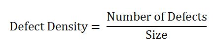
Defect Density is the number of confirmed defects detected in software/component during a defined period of development/operation divided by the size of the software/component.

ELABORATION

The ‘defects’ are:

• confirmed and agreed upon (not just reported).

• Dropped defects are not counted.

The period might be for one of the following:

• for a duration (say, the first month, the quarter, or the year).

• for each phase of the software life cycle.

• for the whole of the software life cycle.

The size is measured in one of the following:

• Function Points (FP)

• Source Lines of Code

DEFECT DENSITY FORMULA

USES

• For comparing the relative number of defects in various software components so that high-risk components can be identified and resources focused towards them.

• For comparing software/products so that quality of each software/product can be quantified and resources focused towards those with low quality.

Defect Removal Efficiency

Definition : The defect removal efficiency (DRE) gives a measure of the development team ability to remove defects prior to release. It is calculated as a ratio of defects resolved to total number of defects found. It is typically measured prior and at the moment of release.

Calculation

To be able to calculate that metric, it is important that in your defect tracking system you track:

• affected version, version of software in which this defect was found.

• release date, date when version was released

DRE = Number of defects resolved by the development team / total number of defects at the moment of measurement.

DRE is typically measured at the moment of version release, the best visualization is just to show current value of DRE as a number.

Example

For example, suppose that 100 defects were found during QA/testing stage and 84 defects were resolved by the development team at the moment of measurement. The DRE would be calculated as 84 divided by 100 = 84%

Test coverage

Test coverage measures the amount of testing performed by a set of test. Wherever we can count things and can tell whether or not each of those things has been tested by some test, then we can measure coverage and is known as test coverage.

The basic coverage measure is where the ‘coverage item’ is whatever we have been able to count and see whether a test has exercised or used this item.

There is danger in using a coverage measure. But, 100% coverage does not mean 100% tested. Coverage techniques measure only one dimension of a multi-dimensional concept. Two different test cases may achieve exactly the same coverage but the input data of one may find an error that the input data of the other doesn’t.

Benefit of code coverage measurement:

• It creates additional test cases to increase coverage

• It helps in finding areas of a program not exercised by a set of test cases

• It helps in determining a quantitative measure of code coverage, which indirectly measure the quality of the application or product.

Drawback of code coverage measurement:

• One drawback of code coverage measurement is that it measures coverage of what has been written, i.e. the code itself; it cannot say anything about the software that has not been written.

• If a specified function has not been implemented or a function was omitted from the specification, then structure-based techniques cannot say anything about them it only looks at a structure which is already there.

Failure Rate

Failure rate is the frequency with which an engineered system or component fails, expressed in failures per unit of time. It is often denoted by the Greek letter λ (lambda) and is highly used in reliability engineering.

The failure rate of a system usually depends on time, with the rate varying over the life cycle of the system. For example, an automobile's failure rate in its fifth year of service may be many times greater than its failure rate during its first year of service. One does not expect to replace an exhaust pipe, overhaul the brakes, or have major transmission problems in a new vehicle.

In practice, the mean time between failures (MTBF, 1/λ) is often reported instead of the failure rate. This is valid and useful if the failure rate may be assumed constant – often used for complex units / systems, electronics – and is a general agreement in some reliability standards (Military and Aerospace). It does in this case only relate to the flat region of the bathtub curve, also called the "useful life period". Because of this, it is incorrect to extrapolate MTBF to give an estimate of the service life time of a component, which will typically be much less than suggested by the MTBF due to the much higher failure rates in the "end-of-life wearout" part of the "bathtub curve".

The reason for the preferred use for MTBF numbers is that the use of large positive numbers (such as 2000 hours) is more intuitive and easier to remember than very small numbers (such as 0.0005 per hour).

The MTBF is an important system parameter in systems where failure rate needs to be managed, in particular for safety systems. The MTBF appears frequently in the engineering design requirements, and governs frequency of required system maintenance and inspections. In special processes called renewal processes, where the time to recover from failure can be neglected and the likelihood of failure remains constant with respect to time, the failure rate is simply the multiplicative inverse of the MTBF (1/λ).

A similar ratio used in the transport industries, especially in railways and trucking is "mean distance between failures", a variation which attempts to correlate actual loaded distances to similar reliability needs and practices.

Failure rates are important factors in the insurance, finance, commerce and regulatory industries and fundamental to the design of safe systems in a wide variety of applications.

Metric examples.pdf